Episode 082, October 2026

Triangle, tamed?

The triangular Hilbert transform at the symmetric point

Covers result 082 in OpenAI’s catalog: all 3 papers. See its connections to other results and the work it cites.

Play Episode 082: Triangle, tamed? A triangle with vertices a, b and c whose three edges are labelled G0(a, b), G1(b, c) and G2(c, a), above the estimate: the L three-halves norm of B(F, G) is at most a constant times the L3 norms of F and G.

5:35. English captions available. The video loads from YouTube when you press play.

Chapters

The claim, in plain words

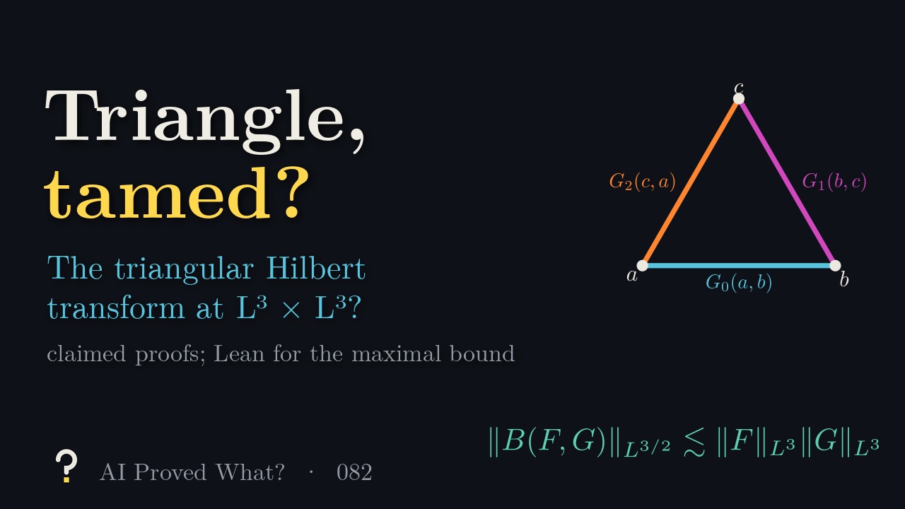
Take two functions F and G on the plane. Read F a distance t to the right and G the same distance up, multiply them, and integrate over t against 1/t, the Hilbert kernel. This is the triangular Hilbert transform; the question is whether it is bounded from L³ × L³ to L^3/2. Pairing with a third function gives a symmetric form in which each of three functions sees one pair of the variables a, b and c, and the three pairs form a triangle. That cycle is what defeats energy methods that telescope across scales for bipartite arrangements; Kovač identified the triangle as an obstacle to his framework.

With the kernel cut to scales between ε and R, earlier bounds grew with the number of scales: Tao proved bounds growing slower than the logarithm for one-dimensional relatives, Zorin-Kranich extended this to the triangle, and Durcik, Kovač and Thiele proved power-type cancellation, which carried to the symmetric point still grows like the square root of log(R/ε). A bound uniform in the scales at the symmetric point is Problem 13 in Thiele’s section of a 2017 problem list, which also asks about a dyadic model.

Result 082 is three OpenAI preprints. The first (27 pages, September 24, 2026) proves the maximal estimate: the supremum over both truncation endpoints, chosen separately at each point, is bounded from L³ × L³ to L^3/2 with an absolute constant, for complex inputs; this gives principal values almost everywhere and in L^3/2, and the symmetric scalar estimate of Thiele’s problem. The second (37 pages, October 5) strengthens this to annular variation bounds for every r > 2, proving all the matrix and heat estimates it needs. The third (11 pages, October 5) bounds the dyadic model: for real inputs, the total of absolute local contributions over any finite set of scales is at most 40 times the product of the norms.

What it doesn’t claim

Only the symmetric point, three equal exponents 3, is claimed; other exponents in the expected range are not.

Where it stands

Posted as preprints: OpenAI, one dated September 24 and two dated October 5, 2026, released October 6
Peer reviewed: Not yet
Checked in Lean: For the maximal estimate only; we have not run the check

Last checked October 19, 2026. None of the three preprints has been revised. OpenAI published a Lean formalization of the first paper’s maximal estimate, 105 files and 10,861 lines with no unproved steps that we could find, matched against a short separate statement with arbitrary complex L³ inputs and the supremum over all finite hard truncations. The variation and dyadic theorems are not formalized, and we have not run the check ourselves. The dyadic paper reuses the first paper’s matrix inequalities and reproduces real-matrix versions of their proofs. None of the papers is among those OSVerify reviewed, and we have seen no expert review.

How the proof goes

Matrices on a triangle. After a change of variables, the inputs become matrices around the triangle of coordinates a, b and c, and a localized piece of the form is a cyclic trace of their product. At each vertex the paper places the two incident matrices side by side as one matrix R and uses the energy tr((R*R)^3/2), which scales like the form. A mixed trace inequality, with constants independent of the matrix size, bounds the cyclic trace by quadratic costs from the Hessians of these energies.
Gaussian heat flow. Integrating the energies over Gaussian centers whose sum is zero, their decrease as the variance grows pays for the quadratic costs at every scale; the total is bounded by the initial energies, which are bounded by sums of cubed L³ norms, so one budget covers all scales.
Switching scales. For the maximal estimate each output point picks its own truncation, so entries of the dual matrix switch on and off and the energy can jump. The total of the jumps is bounded by the L³ masses, through row and column norms and one-dimensional maximal functions; a kernel comparison passes to hard truncations. The variation paper adds a frequency-block estimate and groups endpoints by dyadic radius; the dyadic paper averages the energy over the four children allowed by the binary constraint.

The numbers in the video

A short Python script implements the dyadic form of the third paper on inputs over grids of 8, 16 and 32 cells, counting all scales. It checks the trace formula against a direct sum, gives a one-scale example worth exactly one unit (the product of the three L³ norms), and runs a gradient-ascent search from random starts: the largest ratios found were 1.99, 2.10 and 2.05, far below the paper’s bound of 40. A search is not a proof.

Read the source

The maximal triangular Hilbert transform at the symmetric point (PDF), September 24, 2026 (27 pages).
Annular variation of the triangular Hilbert transform at the symmetric point (PDF), October 5, 2026 (37 pages).
An L³ bound for the dyadic triangular Hilbert form (PDF), October 5, 2026 (11 pages).
The Lean scope note and the statement it is checked against.
The collection’s catalog, where this is result 082.

The 3 papers in this result

OpenAI groups related papers, such as alternative proofs, supporting results and consequences, into one result; we label the first paper it lists the main paper and the others companions.

Annular variation of the triangular Hilbert transform at the symmetric point main paper
An L³ bound for the dyadic triangular Hilbert form companion
The maximal triangular Hilbert transform at the symmetric point companion

Transcript

Read the full script

0:00A triangle of variables

Take two functions F and G on the plane. Read F a distance t to the right, and G the same distance up, multiply them, and integrate over t against 1/t, the Hilbert kernel, which is positive on one side and negative on the other. This is the triangular Hilbert transform. The question is whether it is bounded from L³ times L³ to L^(3/2). Pairing with a third function gives a symmetric form: each of three functions sees one pair of the variables a, b and c, and the three pairs form a triangle. That cycle is what makes the problem hard. Energy methods that telescope across scales work for bipartite arrangements, and Kovač identified the triangle as an obstacle to his framework. With the kernel cut to scales between ε and R, the question is whether the bound can be made independent of the number of scales. Tao proved bounds growing slower than the logarithm for one-dimensional relatives, and Zorin-Kranich extended this to the triangle. Durcik, Kovač and Thiele proved power-type cancellation, but carried to the symmetric point their bound still grows like the square root of the logarithm of R over ε. The symmetric case is Problem 13 in Thiele’s section of a 2017 problem list. Thiele’s problem also asks about a dyadic model, where intervals combine by binary addition without carries. A single dyadic scale contributes at most one unit, the product of the three L³ norms, and our one-scale example reaches it. The question is the total over all scales. We searched for inputs that make the total of absolute contributions as large as possible: on grids of 8, 16 and 32 cells, the largest ratio we found was about two. A search is not a proof.

1:52The claim

Result 082 is three OpenAI preprints. The first, 27 pages, dated September 24, proves the maximal estimate: the supremum over both truncation endpoints, chosen separately at each point, is bounded from L³ times L³ to L^(3/2) with an absolute constant. That gives principal values almost everywhere and in L^(3/2), and the symmetric scalar estimate of Thiele’s problem. The second, 37 pages, dated October 5, strengthens this to an annular variation estimate for every r above two, proving all the matrix and heat estimates it needs. The third, 11 pages, also dated October 5, bounds the dyadic model: the total of absolute local contributions over any finite set of scales, for real inputs, is at most 40 times the product of the norms. OpenAI also published a Lean formalization of the first paper’s maximal estimate, about 11,000 lines in 105 files, matched against a short separate statement with arbitrary complex L³ inputs and the supremum over all finite hard truncations. It does not cover the other two papers. We have not run the check ourselves.

3:11Energy and heat

After a change of variables, the three inputs become matrices around the triangle of coordinates a, b and c, and a localized piece of the form becomes a cyclic trace of their product. At each vertex, the paper places the two incident matrices side by side as one matrix R, and uses the energy: the trace of R*R to the power 3/2, which scales like the form itself. A mixed trace inequality, with constants independent of the matrix size, bounds the cyclic trace by quadratic costs from the Hessians of these energies. Then comes Gaussian heat flow. The paper integrates the energies over Gaussian centers whose sum is zero; as the variance grows, their decrease pays for the quadratic costs at every scale. The total is bounded by the initial energies, which are bounded by sums of cubed L³ norms, so one budget covers all scales at once. For the maximal estimate, each output point picks its own truncation, so entries of the dual matrix switch on and off at their own scales, and the energy can jump. The key new estimate bounds the total of these jumps by the L³ masses: the derivative in one entry is controlled by its row and column norms, and one-dimensional maximal functions control those uniformly in the switching scales. A comparison of kernels then passes from smooth to hard truncations. The variation paper adds a frequency-block estimate and groups hard endpoints by dyadic radius. The dyadic paper averages the same energy over the four children allowed by the binary constraint.

4:49Where it stands

None of the three preprints is peer reviewed, and none has been revised. The maximal estimate has a Lean formalization, which we have not run; the variation and dyadic theorems do not. The dyadic paper takes its matrix inequalities from the first paper and reproduces real-matrix versions of their proofs. None of the three is among the papers OSVerify reviewed, and we have seen no expert review. If they hold, the triangular Hilbert transform is bounded at the symmetric point, with maximal and variation bounds and principal values, and the dyadic model is bounded at the same exponents. Other exponents in the expected range are not claimed.

Spot a mistake?

This episode simplifies on purpose, but it shouldn’t be wrong. If something is, open an issue on GitHub or leave a comment on YouTube. Corrections are noted here with a date.