Three shifts, one bound?
An L3 bound for the trilinear Hilbert transform
Covers result 086 in OpenAI’s catalog: its one paper. See its connections to other results and the work it cites.
6:05. English captions available. The video loads from YouTube when you press play.
Chapters
The claim, in plain words
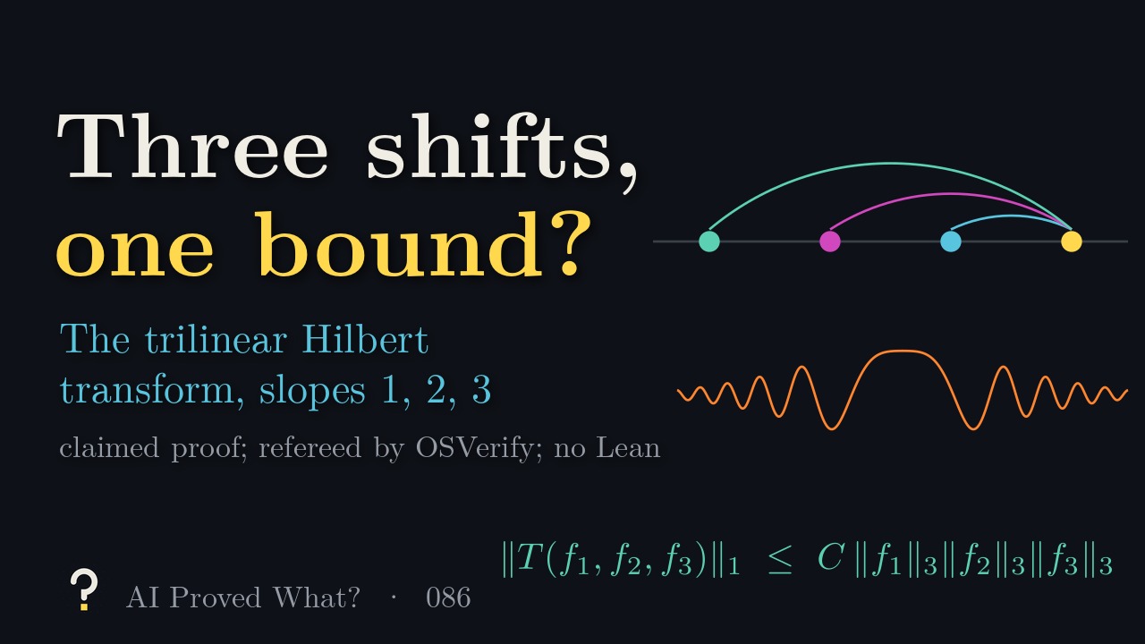
Take three functions on the line. At each point x, multiply the first at x − t, the second at x − 2t and the third at x − 3t, and integrate against 1/t, the kernel of the Hilbert transform, as a principal value. This is the trilinear Hilbert transform T. Scaling pairs three inputs in L3 with an output in L1, since 1/3 + 1/3 + 1/3 = 1.
With two functions this is the bilinear Hilbert transform from Calderón’s work, bounded by Lacey and Thiele in 1997 and 1999 using time-frequency analysis. That transform is symmetric under matched linear waves. Three functions bring a quadratic symmetry: the coefficients −1, 3, −3, 1 cancel every constant, line and parabola along x, x − t, x − 2t, x − 3t, so matched quadratic waves pass through, and the output only picks up a quadratic wave. Wave packets built on linear frequencies are not adapted to this symmetry. Each scale on its own is easy; cutting the kernel to N scales, the elementary bound grows in proportion to N, and in 2015 Tao used higher-order Fourier analysis to show it grows more slowly than that. Hu and Lie proved bounds for curved versions; for straight lines with slopes 1, 2 and 3, boundedness remained open in their account.
Result 086 is one OpenAI preprint, 93 pages, dated October 5, 2026. Its theorem: there is a finite constant C such that ‖T(f1, f2, f3)‖1 ≤ C ‖f1‖3 ‖f2‖3 ‖f3‖3, so T extends to a bounded map from L3 × L3 × L3 to L1. The paper presents this as resolving the L3 case of the trilinear Hilbert transform conjecture for slopes 1, 2 and 3.
What it doesn’t claim
The conjecture asks for a broader range of exponents, and other slopes are not treated. The constant is not computed. Transforms with more functions are not claimed.
Where it stands
- Posted as a preprint
- OpenAI, dated October 5, 2026, released October 6
- Peer reviewed
- Not yet
- Checked in Lean
- No Lean formalization published
Last checked October 19, 2026. The preprint has not been revised, and OpenAI published no Lean formalization of this result. OSVerify refereed the paper (the October 5 version) and reported one major issue and two minor ones, each with a proposed repair. The major one: Lemma 8.6, a counting lemma for bad-density chains, states its nesting hypothesis only before the last position, but the proof uses it at the last one too; the proposed repair leaves the lemma’s bound unchanged, and where the lemma is applied both inclusions are available. The minor ones: an identity in the proof of Lemma 5.3 omits a conditional-expectation term for general inputs, and a convention in Section 9.1 is stated in the wrong order. The report says its findings “do not necessarily establish that the paper’s main theorem is false.” We have seen no other expert review.
How the proof goes
- Absorbing the scales. A fourth function turns T into a four-linear form, split into local pieces on dyadic intervals, with kernels that integrate to zero whenever any one of the four points is held fixed. A stopping argument with a maximal function reduces everything to one estimate: on a normalized tree, the length-weighted sum of the pieces is at most the root’s length times A + c·CN, where CN is the best constant for N scales. Since CN is finite (at most of order N), a small c can be absorbed, and the bound no longer depends on N.
- Structure at one scale. A large local form forces one of the inputs to correlate with a generalized quadratic phase. The paper uses the degree-two case of the quantitative inverse theorem of Leng, Sah and Sawhney for Gowers norms, and proves the continuous chart and localization statements the singular integral needs. Private orthogonal coordinates make the coefficients of each selected column recoverable, and a compression lemma controls products of inherited projections uniformly in depth, at the cost of a power of a logarithm.
- Gains against losses. Curvature is localized jointly in all four arguments, and a short-block comparison costs only a small power of the block length. Each matched column gets one fixed mode expansion; frequency graphs separate errors with square-summable energy from coherent components; and a counting lemma, applied with all four cancellations, bounds the total mass of progression tests on scales of small density with a power saving. The parameters are chosen so that every gain beats every loss, and the absorption closes.
The numbers in the video
- A short Python script confirms that the coefficients −1, 3, −3, 1 cancel constants, lines and parabolas but not cubes, while 1, −2, 1 cancel only constants and lines.
- With three Gaussian inputs, the trilinear output has L1 norm 2.9753. After matched quadratic waves of strength 0.5, 1 and 2 the output changes only by a quadratic wave, pointwise to rounding, so its L1 norm stays 2.9753. For the bilinear transform with two of the same Gaussians, matched linear waves leave the L1 norm at 4.33, while matched quadratic waves shrink it to 1.89, 1.34 and 0.95. No computation can test every input.
Read the source
- An L3 bound for the trilinear Hilbert transform (PDF), October 5, 2026 (93 pages).
- The OSVerify referee report.
- The collection’s catalog, where this is result 086.
The paper
OpenAI groups related papers into one result; this one has a single paper.
Transcript
Read the full script
0:00Three shifted copies
Take three functions on the line. At each point x, multiply the first at x − t, the second at x − 2t, and the third at x − 3t, and integrate against 1/t, the kernel of the Hilbert transform, cutting out a small symmetric interval around zero and letting it shrink. This is the trilinear Hilbert transform. Scaling pairs three inputs in L³ with an output in L¹, since 1/3 + 1/3 + 1/3 = 1. The question is whether the output’s L¹ norm is at most a constant times the product of the three L³ norms. With two functions, this is the bilinear Hilbert transform from Calderón’s work, bounded by Lacey and Thiele in 1997 and 1999 using time-frequency analysis. That transform has a symmetry: multiply the inputs by matched linear waves, and the output only picks up a wave. Three functions bring a larger symmetry. The coefficients −1, 3, −3, 1 cancel every constant, line and parabola along the points x, x − t, x − 2t, x − 3t. So matched quadratic waves, of any strength, pass through: the output only picks up a quadratic wave, and its size does not change. In our computation, with three Gaussian inputs, the output’s L¹ norm stays at about 2.98, unchanged up to rounding, as the waves get faster; the same kind of quadratic wave shrinks the bilinear output from 4.33 to about 0.95. Wave packets built on linear frequencies are not adapted to this quadratic symmetry, so the methods that worked for two functions do not carry over. Each scale on its own is easy; the trouble is the sum over scales. Cutting the kernel to N scales, the elementary bound grows in proportion to N. In 2015, Tao used higher-order Fourier analysis to show it grows more slowly than that. Hu and Lie proved bounds for curved versions, where the curvature supplies a different kind of oscillation. For straight lines with slopes one, two and three, boundedness remained open, in Hu and Lie’s account.
2:15The claim
Result 086 is a 93-page OpenAI preprint dated October 5. Its theorem: there is a finite constant C such that the L¹ norm of the trilinear Hilbert transform is at most C times the product of the three L³ norms, so the transform extends to a bounded map from three copies of L³ to L¹. The paper presents this as resolving the L³ case of the trilinear Hilbert transform conjecture for slopes one, two and three. Nothing more is claimed. The conjecture asks for a broader range of exponents, and other slopes are not treated. The constant is not computed. OpenAI published no Lean formalization of this result.
2:59Summing the scales
The proof adds a fourth function and studies the four-linear form, split into local pieces on dyadic intervals, with kernels that integrate to zero whenever any one of the four points is held fixed. A stopping argument with a maximal function reduces everything to one estimate: on a normalized tree, the sum of the pieces, weighted by their lengths, is at most the root’s length times a constant A plus a small multiple c of the best constant for N scales. That constant is finite, at most of order N, so the small multiple can be absorbed, and the bound no longer depends on N. At one scale, a large local form forces one of the inputs to correlate with a generalized quadratic phase. The paper uses the degree-two case of the quantitative inverse theorem of Leng, Sah and Sawhney for Gowers norms, and proves the continuous chart and localization statements the singular integral needs. Private orthogonal coordinates make the coefficients of each selected column recoverable, and a compression lemma controls products of inherited projections uniformly in depth, at the cost of a power of a logarithm. The inverse theorem alone does not sum the scales. Curvature is localized jointly in all four arguments, and a short-block comparison costs only a small power of the block length. Each matched column gets one fixed mode expansion; frequency graphs separate errors with square-summable energy from coherent components; and a counting lemma, applied with all four cancellations, bounds the total mass of progression tests on scales of small density, with a power saving. The parameters are then chosen so that every gain beats every loss, and the absorption closes.
4:46Where it stands
The preprint is not peer reviewed, has not been revised, and has no Lean formalization. OSVerify reviewed it and reported one major issue and two minor ones. The major one: Lemma 8.6, a counting lemma for bad-density chains, states its nesting hypothesis only before the last position, but the proof uses it at the last one too. The report proposes a repair that leaves the lemma’s bound unchanged, and notes that where the lemma is applied, both inclusions are available. The minor ones: an identity in the proof of Lemma 5.3 omits a conditional-expectation term for general inputs, and a convention in Section 9.1 is stated in the wrong order. Each has a proposed fix, and the report says its findings do not necessarily show the main theorem is false. We have seen no other expert review. If it holds, the trilinear Hilbert transform with slopes one, two and three is bounded from three copies of L³ to L¹, settling a case that, in Hu and Lie’s account, had remained open, even though matched quadratic waves leave the size of its output untouched. Other exponents, other slopes, and transforms with more functions are not claimed.
Spot a mistake?
This episode simplifies on purpose, but it shouldn’t be wrong. If something is, open an issue on GitHub or leave a comment on YouTube. Corrections are noted here with a date.