Episode 122, October 2026

Polynomially many traces?

A claimed superpolynomial lower bound for trace reconstruction, and a uniform quasipolynomial decoder

Covers result 122 in OpenAI’s catalog: all 3 papers. See its connections to other results and the work it cites.

Play Episode 122: Polynomially many traces? A binary string with deleted bits and the traces that remain.

7:06. English captions available. The video loads from YouTube when you press play.

Chapters

The claims, in plain words

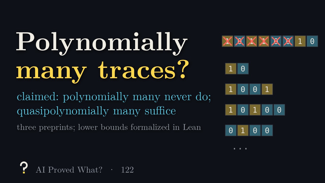
Take a binary string, delete each bit independently with a fixed probability, and glue the survivors together. That is a trace: you see its length and its bits, but not where they came from. Trace reconstruction asks how many independent traces it takes to recover every string of length n with high probability, knowing n and the deletion probability. The known hard cases are strings that differ only by a small shift.

Batu, Kannan, Khanna and McGregor posed the problem in its modern form, motivated by sequence alignment. At a fixed deletion probability, upper bounds came down from exp(Õ(√n)) traces (Holenstein, Mitzenmacher, Panigrahy and Wieder) to exp(O(n^1/3)) (De, O’Donnell and Servedio; Nazarov and Peres) and exp(Õ(n^1/5)) (Chase). A 2026 preprint by Burudgunte, Valiant and Wang, cited by these papers, reached a quasipolynomial number of traces, with an unspecified power of log n, but no quasipolynomial-time algorithm. Lower bounds stood near n^5/4 (Holden and Lyons) and n^3/2 (Chase). Whether polynomially many traces always suffice was open.

Result 122 is three OpenAI preprints. The first (42 pages, September 24, 2026) claims that at every fixed deletion probability q, exact reconstruction of every binary string of length n needs at least n^{c log(q³ log n)} traces for every c below 1/(4 log 2), once n is large enough: n^{Ω(log log n)}, even with unlimited computation and any fixed positive chance of success. So polynomially many traces never suffice. It also claims that, for large n, some two different strings have single-trace laws closer in total variation than any fixed inverse power of n.

The second (29 pages, October 5, 2026) gives one randomized algorithm that, knowing n and a rational retention probability (one minus the deletion probability), recovers any string with probability at least 2/3. At a fixed retention probability it uses exp(C (log n)³ (log log n)⁶) traces with quasipolynomial bit complexity; when the deletion probability is at most n^−ε, both bounds become polynomial. The third (15 pages, October 5, 2026) proves the same sample bound, also for general symbols, with no efficient algorithm.

What they don’t claim

The lower bound is about growth, not size: its constant is small, and at deletion probability 1/2 the formula passes Chase’s exponent 3/2 only once n has more than 220 digits; the theorem only says “eventually”. A gap remains between the bounds: the logarithm of the number of traces is between order log n · log log n and (log n)³, up to log log factors. The decoder needs the retention probability as a known rational number.

Where it stands

Posted as preprints: OpenAI, three preprints: 42 pages (September 24, 2026), 29 and 15 pages (October 5, 2026)
Peer reviewed: Not yet
Checked in Lean: OpenAI published a Lean proof of the lower bounds; the upper bounds are not formalized; we have not run the check

Last checked October 19, 2026. The preprints have not been revised. OpenAI published a Lean formalization of the lower bounds (the quantitative bound, superpolynomial one-trace indistinguishability and superpolynomial sample complexity), stated for every estimator with unlimited computation and matched against its comparator statement, in 31 files and 33,984 lines with its imports (not counting Mathlib), with no unproved steps that we could find. We have not run the check. The upper bounds are not formalized. None of the papers is among those OSVerify reviewed, and we have seen no expert review.

How it works

Hiding a shift. If the traces of k copies of a word and of k + 1 copies share some mass, place such a pair of runs on both sides of a central segment and let a fair coin decide which side gets the extra copy. On the shared part the coin stays hidden even after the outputs are seen, and many independent pairs leave the central segment at a binomially random offset.
Signs that cancel. The two words differ in their central segments by complementary Prouhet–Thue–Morse signed patterns (plus, minus, minus, plus, then that block with every sign flipped, and so on). The generating polynomial vanishes to high order at 1, so after averaging over the broad offset the difference nearly cancels.
Climbing scales. A hard pair at one length becomes the building block for a much longer pair. The proof tracks a likelihood score on auxiliary laws that turn into genuine traces up to small, recorded errors; each low-degree term of the score difference cancels between the two words, is smoothed away by the signs, or forces a binary tree of earlier score factors. A level of depth B raises the sample exponent by about (B − 1)/4, and there are about log log n/(B log 2) levels.
A decoder, bit by bit. The decoder estimates products of trace bits at chosen ranks and tests each guess for the next bit by asking whether a positive moment array for the remaining bits, in the style of Lasserre’s relaxations, matches the estimates. The key theorem separates the true string from every such array that fixes a wrong prefix, pushing the signal at the first wrong bit through larger scales and then, by a generating-function identity, to trace statistics. The true prefix has slack, so finitely many exact rational updates find a feasible array.

The numbers in the video

Exact one-trace laws for every pair of binary strings up to length 10, deletion probability 1/2: the closest pairs at length 10 are a single one, or a single zero, moved by one place in the middle, at total variation 63/512 ≈ 0.123.
Runs of 100 and 101 zeros have trace laws sharing 96% of their mass; runs of 10,000 and 10,001 share 99.6%.
Against a binomial offset with 40,000 steps, a single sign leaves a signal of 0.004; the Thue–Morse pattern of length 32 leaves about 2 billionths.
At deletion probability 1/2, even with c at its limit 1/(4 log 2), the exponent is at most 0.20 at n = 10⁶ and 1.21 at n = 10¹⁰⁰, passing 3/2 only for n beyond 10²²².

Read the source

Quantitative lower bounds for trace reconstruction (PDF), 42 pages.
Uniform quasipolynomial-time trace reconstruction (PDF), 29 pages.
A latest-anchor induction with spectrally compact masks for worst-case trace reconstruction (PDF), 15 pages.
The Lean scope note.
The collection’s catalog, where this is result 122.

The 3 papers in this result

OpenAI groups related papers, such as alternative proofs, supporting results and consequences, into one result; we label the first paper it lists the main paper and the others companions.

Uniform quasipolynomial-time trace reconstruction main paper
A latest-anchor induction with spectrally compact masks for worst-case trace reconstruction companion
Quantitative lower bounds for trace reconstruction companion

Transcript

Read the full script

0:00Traces

Take a binary string, delete each bit independently with some fixed probability, say 1/2, and glue the survivors together. That is a trace: you see its length and its bits, but not where they came from. Trace reconstruction asks how many independent traces it takes to recover every string of length n, with high probability, knowing n and the deletion probability. The known hard cases are strings that differ only by a small shift. In our check of every pair of strings up to length 10, the closest pairs at length 10 are a single one, or a single zero, moved by one place in the middle, and the trace laws of the two differ in total variation by only about 1/8. Batu, Kannan, Khanna and McGregor posed the problem in its modern form, motivated by sequence alignment. At a fixed deletion probability, upper bounds came down from exp(√n), up to logarithms, by Holenstein, Mitzenmacher, Panigrahy and Wieder, to exp(n^(1/3)), by De, O’Donnell and Servedio and by Nazarov and Peres, and to exp(n^(1/5)), up to logarithms, by Chase. A 2026 preprint by Burudgunte, Valiant and Wang, cited by these papers, reached a quasipolynomial number of traces, with an unspecified power of log n, but no quasipolynomial-time algorithm. Lower bounds were far smaller: Holden and Lyons proved about n^(5/4), and Chase about n^(3/2). Whether polynomially many traces always suffice was open.

1:33The claims

Result 122 is three OpenAI preprints. The first, 42 pages, dated September 24, claims that at every fixed deletion probability, exact reconstruction of every binary string of length n needs at least n^(c log log n) traces, even with unlimited computation and any fixed positive chance of success. So polynomially many traces never suffice. More precisely, the bound is n^(c log(q³ log n)), for every c below 1/(4 log 2), once n is large enough, where q is the deletion probability. It also claims that, for large n, some two different strings have single-trace laws closer in total variation than any fixed inverse power of n. Two companions, dated October 5, go the other way. One, 29 pages, gives a single randomized algorithm that, knowing n and a rational retention probability, one minus the deletion probability, recovers any string with probability at least 2/3. At a fixed retention probability, the number of traces is exp(C (log n)³ (log log n)⁶), and the bit complexity is quasipolynomial. When the deletion probability is at most n^(−ε), both bounds become polynomial. The other, 15 pages, proves the same sample bound, with no efficient algorithm, and also for larger alphabets. A gap remains in the exponent. OpenAI published a Lean formalization of the lower bounds, 31 files and about 34,000 lines with its imports, not counting Mathlib. The upper bounds are not formalized.

3:18How it works

The lower bound hides differences in position at many scales. It starts from common mass: if the traces of k copies of a word and of k + 1 copies share mass ω, place such a pair of runs on both sides of a central segment, and let a fair coin decide which side gets the extra copy. On the shared part, the coin stays hidden even after the outputs are seen, and many independent pairs leave the central segment at a binomially random offset. In our check, at retention one half, runs of 100 and 101 zeros share 96% of their trace mass, and runs of 10,000 and 10,001 share 99.6%. The two words differ in their central segments by complementary signed patterns, taken from the Prouhet–Thue–Morse sequence: plus, minus, minus, plus, then that block with every sign flipped, and so on, doubling the length each time. Its generating polynomial vanishes to high order at one, so after averaging over a broad random offset, the difference nearly cancels. In our check, with an offset spread like a binomial with 40,000 steps, a single sign leaves a signal of 0.004, while the Thue–Morse pattern of length 32 leaves about 2 billionths. The construction is recursive. A hard pair at one length becomes the building block for a much longer pair, and the proof tracks a likelihood score on auxiliary laws that turn into genuine traces up to small, recorded errors. Each low-degree term of the score difference either cancels between the two words, is smoothed away by the signs, or forces a binary tree of earlier score factors. A level of depth B raises the sample exponent by about (B − 1)/4, and there are about log log n/(B log 2) levels, so, with B large, the exponent gets close to log log n/(4 log 2). That constant is small: at deletion probability one half, the formula passes Chase’s 3/2 only once n has more than 220 digits, and the theorem only says eventually. The point is the growth. The decoder works one bit at a time. It estimates products of trace bits at chosen ranks, which may be far apart, and tests each guess for the next bit by asking whether some positive moment array for the remaining bits, in the style of Lasserre’s relaxations, matches the estimates. The key theorem separates the true string from every such array that fixes a wrong prefix. It pushes the signal at the first wrong bit through larger and larger scales, using positivity, damped Fourier sums and a Gaussian contour shift, then a generating-function identity carries it from input statistics to trace statistics. The true prefix has slack, so finitely many exact rational updates find a feasible array, and the running time is polynomial in the sample budget.

6:15Where it stands

The three preprints are not peer reviewed and have not been revised. The Lean formalization covers the lower bounds, stated for every estimator with unlimited computation; we have not run it. The upper bounds are not formalized. None of the papers is among those OSVerify reviewed, and we have seen no expert review. If they hold, trace reconstruction needs superpolynomially many traces at every fixed deletion probability, answering the polynomial question in the negative, while quasipolynomially many suffice, now with an explicit exponent and, for rational probabilities, a decoder to match. What remains is the gap in the logarithm of the number of traces: between log n · log log n and (log n)³, up to log log factors.

Spot a mistake?

This episode simplifies on purpose, but it shouldn’t be wrong. If something is, open an issue on GitHub or leave a comment on YouTube. Corrections are noted here with a date.