How long is a random curve?
Two preprints claim an exact Hausdorff gauge for SLE, answering Schramm’s question
Covers result 230 in OpenAI’s catalog: all 2 papers. See its connections to other results and the work it cites.
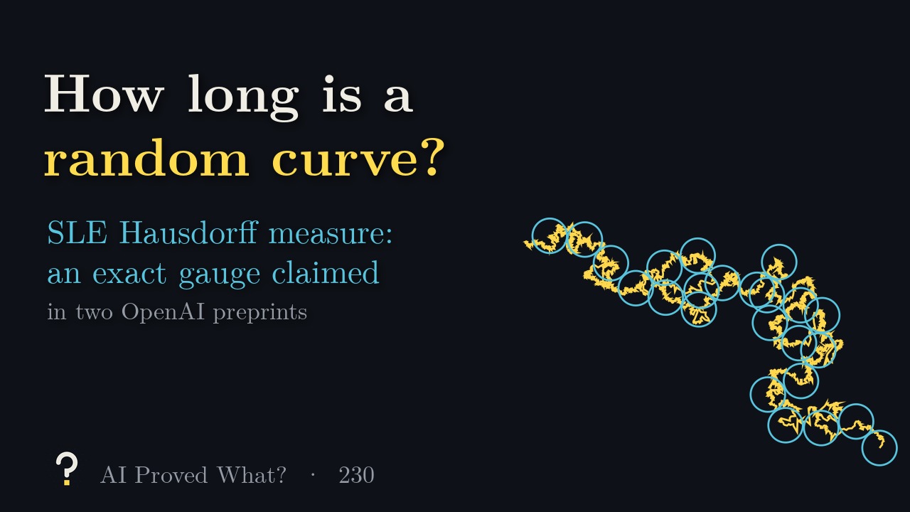
4:35. English captions available. The video loads from YouTube when you press play.
Chapters
The claim, in plain words
Schramm–Loewner evolution (SLE) is a family of random curves in the plane, indexed by a number κ, that describe boundaries in many two-dimensional models at criticality, such as percolation clusters and Ising spin clusters. For κ between 0 and 8, Vincent Beffara proved in 2008 that the curve has dimension d = 1 + κ/8: its length is infinite and its area zero. The natural way to measure it is Hausdorff measure: cover the curve with small pieces, charge each a cost h(r) depending on its size (the gauge), and take the cheapest cover. A gauge is exact if the answer is neither zero nor infinite. The obvious gauge rd gives zero (Rezaei, 2018). In 2006 Oded Schramm asked for a σ-finite Hausdorff measure on the SLE path, and expected the gauge rd log log(1/r).
Result 230 is two OpenAI preprints, 86 pages, dated September 25 and 26, 2026. The first claims that for every κ below 8 some exact gauge exists, built from moments of a local mass, with no closed formula. The second claims an explicit one, h(r) = rd (log log 1/r)(2−d)/2: almost surely every piece of the curve after time zero gets positive, finite measure, and the expected measure in any bounded disk is finite. It also shows Schramm’s guess was too big: with exponent one, every piece of the curve has measure that is not even σ-finite.
What it doesn’t claim
That the new measure equals the curve’s natural length (built by Lawler with Sheffield, Zhou and Rezaei), or that the two papers’ gauges agree; both papers say the relation between the gauges remains open. Only chordal SLE is covered, from one boundary point to another, for fixed κ below 8.
Where it stands
- Posted as preprints
- OpenAI, two papers, 86 pages, dated September 25 and 26, 2026
- Peer reviewed
- Not yet
- Checked in Lean
- In part (docs)
Last checked October 19, 2026. Neither preprint has been revised since release. In Lean, the one listed comparator checks only the positive lower bound for the explicit gauge; the Lean folders also contain the full theorems with no unproved steps, but they are not catalogued, and we did not build them. On October 10, 2026, Dapeng Zhan posted a short paper (arXiv 2610.15066) that takes the explicit theorem as an input and shows the new measure is a constant times natural length; he says he used GPT 6 to explore proof ideas, and checked the details himself. Neither paper is among those OSVerify reviewed.
How the proof goes
- Lower bound. The mass of the curve in a small disk has a tail that falls off like exp(−u2/(2−d)). Over about log(1/r) scales, the worst excess you meet grows like (log log 1/r)(2−d)/2. Delete the rare overfull squares, and what is left spreads its mass no faster than the gauge.
- Upper bound. A matching rare event: a serpentine ribbon where the curve winds back and forth m times, with probability about e−m² and extra mass m2−d. Choosing m like √(log n) balances the two, and both sides give the same exponent. The hard part is making each step hold uniformly over every rough past of the curve.
The numbers in the video
- Ours: simulated SLE curves (Loewner equation, 20,000 steps) for κ = 2, 4, 6; box-counting slopes 1.22, 1.39, 1.52 against the true 1.25, 1.5, 1.75 (the right order, but low, as box counts over two decades of scale tend to be).
- Ours: the size of the correction. For κ = 4, measuring in meters, even at the Planck length the factor (log log 1/r)1/4 is only about 1.45; reaching a factor of two needs 1/r ≈ 103.9 million.
Read the source
The 2 papers in this result
OpenAI groups related papers, such as alternative proofs, supporting results and consequences, into one result; we label the first paper it lists the main paper and the others companions.
- An exact Hausdorff gauge for SLE main paper
- An explicit exact Hausdorff gauge for SLE companion
Transcript
Read the full script
0:00The question
How long is a random fractal curve? Schramm–Loewner evolution, SLE, is a family of random curves in the plane, indexed by a number κ. They describe the boundaries in many two-dimensional models at criticality, such as percolation clusters and Ising spin clusters. For κ between zero and eight, Vincent Beffara proved in 2008 that the curve has dimension one plus κ over eight: more than a line, less than an area. So its ordinary length is infinite, and its area is zero. The natural way to measure such a curve is Hausdorff measure. Cover the curve with small pieces, charge each piece a cost that depends on its size, called the gauge, and take the cheapest cover. A gauge is exact if the answer is neither zero nor infinite. The obvious gauge, r to the power d, gives zero: Rezaei proved this in a paper published in 2018. In 2006, Oded Schramm asked for a Hausdorff measure on the SLE path that is sigma-finite, and he expected the gauge r to the d times log log of one over r, based on experience with similar random paths.
1:11The claim
Result 230 is two OpenAI preprints, 86 pages, dated September 25 and 26, 2026. The first claims that, for every κ below eight, some exact gauge exists, built from moments of a local mass, with no closed formula. The second claims an explicit one: r to the d, times log log of one over r, raised to the power two minus d, over two. Almost surely, every piece of the curve after time zero gets positive, finite measure, and the expected measure in any bounded disk is finite. It also shows that Schramm’s guess was too big: with exponent one, every piece of the curve has measure that is not even sigma-finite. Not claimed: that the new measure equals the curve’s natural length, built by Lawler with Sheffield, Zhou and Rezaei, or that the two papers’ gauges agree. Both papers say the relation between their gauges remains open. Only chordal SLE is covered, from one boundary point to another.
2:14How the proof goes
Why log log? The mass of the curve in a small disk has a tail that falls off like e to the minus u to the power two over two minus d. Over about log of one over r scales, the worst excess you meet grows like log log of one over r, to the power two minus d, over two. That gives the lower bound: delete the rare overfull squares, and what is left spreads its mass no faster than the gauge. For the upper bound, the paper builds the matching rare event: a serpentine ribbon, where the curve winds back and forth m times. That costs probability about e to the minus m squared, and gains mass m to the power two minus d. Choosing m like the square root of log n balances the two, and both sides give the same exponent. The hard part is making each step hold uniformly over every rough past of the curve. As an illustration, our computer simulated the curves for κ two, four and six. Box counting gives slopes of about 1.22, 1.39 and 1.52, against the true 1.25, 1.5 and 1.75: the right order, but low, as box counts over two decades of scale tend to be. And the correction is tiny. For κ four, measure in meters: even at the Planck length the factor is only about 1.45. Reaching a factor of two needs one over r of 10^(nearly 4 million). No simulation could ever see it.
3:43Where it stands
Both preprints are unrefereed and unchanged since release. In Lean, the one listed comparator checks only the positive lower bound for the explicit gauge; the Lean folders also contain the full theorems, sorry-free, but they are not catalogued, and we did not build them. On October 10, Dapeng Zhan posted a short paper that takes the explicit theorem as an input and shows the new measure is a constant times natural length; he says he used GPT 6 to explore proof ideas, and checked the details himself. Neither paper is among those OSVerify reviewed. If they hold, Schramm’s twenty-year-old question has an answer, with a formula, and his guessed exponent of one was too large: for SLE with κ four, it is one quarter.
Spot a mistake?
This episode simplifies on purpose, but it shouldn’t be wrong. If something is, open an issue on GitHub or leave a comment on YouTube. Corrections are noted here with a date.