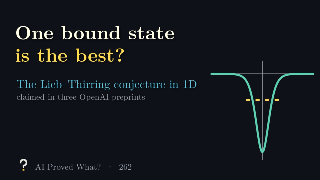
One bound state is the best?
Three AI preprints claim the one-dimensional Lieb–Thirring conjecture, for scalar and matrix wells
Covers result 262 in OpenAI’s catalog: all 3 papers. See its connections to other results and the work it cites.
3:47. English captions available. The video loads from YouTube when you press play.
Chapters
The claim, in plain words
Put a quantum particle on a line, in a potential well. It can sit in a few bound states, each with a negative energy. Lieb and Thirring bounded the sum of the sizes of those energies, each raised to a power γ, by a constant times an integral of the well’s depth to the power γ + 1/2. Their three-dimensional version gave a short proof that ordinary matter is stable.
What is the best constant? In one dimension, above γ = 3/2, a crowd of states wins; that was known by 1978. For γ between 1/2 and 3/2, Lieb and Thirring conjectured in 1976 that the best well holds a single bound state, a soliton-shaped well. The lower end was proved in 1998, but a 2020 survey by Frank called the middle range open. At γ = 1 the best proved constant was about 1.45 times the classical one, against a conjectured 1.15.
Result 262 is three OpenAI preprints, 73 pages in all. The first, 21 pages, dated September 23, 2026, claims the conjecture for every γ strictly between 1/2 and 3/2. The case γ = 1 had been posted on September 9 by Larry Read, then with Marvin Schulz, and the OpenAI paper credits it; Read’s own paper says a first version of its proof was developed by an AI model. The second, 24 pages, dated October 5, claims the same constant for wells whose depth is a matrix of any finite size, even when the matrices do not commute. The third, 28 pages, claims that equality holds only for independent soliton wells, one per channel, in one fixed basis.
What it doesn’t claim
Anything in higher dimensions, or values of γ outside the open range.
Where it stands
- Posted as preprints
- OpenAI, three papers, 21, 24 and 28 pages, dated September 23 and October 5, 2026
- Peer reviewed
- Not yet
- Formalized in Lean
- The scalar theorem in full (docs)
Last checked October 19, 2026. The preprints have not been revised. In Lean, the scalar theorem is formalized in full: about 13,700 lines with no unproved steps, which we did not build. The matrix and equality papers are not formalized. OSVerify has not reviewed them, and we found no specialist comment.
How the proofs go
- A path through matrices. The key move walks a symmetric matrix from one value to its negative along a differential equation, and a parity count shows such a path exists. Integrating along it gives each bound state exactly its single-state share.
- Matrix wells. The new ingredient is a trace inequality comparing two matrix quantities. It lets the scalar argument go through even when the matrices share no common basis.
The numbers in the video
- Ours: with exact soliton wells, the single-state well wins below 3/2, every reflectionless well ties at exactly 3/2, and at γ = 2 wells with many states beat it by about 7%. Of 3,000 random wells, none beat the single-state constant at five sampled values of γ below 3/2.
- Ours: twisting the basis of a matrix well along the line lowers the ratio, to about 93% at one twist rate and 70% at four times that rate.
- Ours: a naive optimizer seemed to beat the theorem by 27%, using a spike thinner than its grid. Resolved properly, at γ = 1, it reached 99.8% and never more.
Read the source
- Sharp One-Dimensional Lieb–Thirring Constants (PDF), 21 pages.
- Sharp One-Dimensional Lieb–Thirring Inequalities for Matrix Potentials (PDF), 24 pages.
- Equality Cases in the Sharp One-Dimensional Matrix Lieb–Thirring Inequality (PDF), 28 pages.
- Read and Schulz, arXiv 2609.10478, the case γ = 1.
- The Lean formalization notes.
- The collection’s catalog, where this is result 262.
The 3 papers in this result
OpenAI groups related papers, such as alternative proofs, supporting results and consequences, into one result; we label the first paper it lists the main paper and the others companions.
Transcript
Read the full script
0:00The question
Put a quantum particle on a line, in a potential well. It can sit in a few bound states, each with a negative energy. Lieb and Thirring bounded the sum of the sizes of those energies, each raised to a power γ, by a constant times an integral of the well’s depth to the power γ + 1/2. Their three-dimensional version gave a short proof that ordinary matter is stable. What is the best constant? In one dimension, above 3/2, a crowd of states wins; that was known by 1978. For gamma between 1/2 and 3/2, Lieb and Thirring conjectured in 1976 that the best well holds a single bound state, a soliton-shaped well. The lower end was proved in 1998, but a 2020 survey by Frank called the middle range open. At γ = 1, the best proved constant was about 1.45 times the classical one, against a conjectured 1.15. Our computer checks the picture with exact soliton wells: below 3/2 the single-state well wins; at exactly 3/2 every reflectionless well ties; at γ = 2, wells with many states beat it by about 7%. Of 3,000 random wells, none beat the single-state constant at five values of γ below 3/2.
1:21The claims
Result 262 is three OpenAI preprints, 73 pages in all. The first, 21 pages, dated September 23, 2026, claims the conjecture for every γ strictly between 1/2 and 3/2. The case γ = 1 had been posted on September 9 by Larry Read, then with Marvin Schulz, and the OpenAI paper credits it; Read’s own paper says a first version of its proof was developed by an AI model. The second, 24 pages, dated October 5, claims the same constant for wells whose depth is a matrix of any finite size, even when the matrices do not commute. The third, 28 pages, claims that equality holds only for independent soliton wells, one per channel, in one fixed basis. Our check: twisting the basis along the line lowers the ratio, to about 93% at one twist rate and 70% at four times that rate. Not claimed: anything in higher dimensions, or values of γ outside the open range. Numerics can mislead here: our naive optimizer seemed to beat the theorem by 27%, using a spike thinner than its grid. Resolved properly, at γ = 1, it reached 99.8% and never more.
2:44How the proofs go
The key move walks a symmetric matrix from one value to its negative along a differential equation, and a parity count shows such a path exists; integrating along it gives each bound state exactly its single-state share. For matrix wells the new ingredient is a trace inequality comparing two matrix quantities, which lets the scalar argument go through even when the matrices share no common basis.
3:09Where it stands
The preprints are unrefereed and unchanged since release. In Lean, the scalar theorem is formalized in full, about 13,700 lines with no unproved steps, which we did not build; the matrix and equality papers are not formalized. OSVerify has not reviewed them, and we found no specialist comment. If they hold, a 50-year-old guess about wells on a line is settled: between 1/2 and 3/2, one bound state is the most efficient way to bind, for scalars and finite matrices alike.
Spot a mistake?
This episode simplifies on purpose, but it shouldn’t be wrong. If something is, open an issue on GitHub or leave a comment on YouTube. Corrections are noted here with a date.